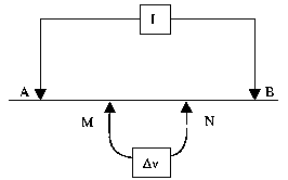
Electric prospection is based on rocks resistivity (electricity carrying ease) measure (ρ). there are two kinds of electric measures : vertical and horizontal. Both measures are based on the same protocole. Two electric measures electrodes (M and N) locate between two electric current injections electrodes (A and B).
For the vertical measures, electrodes M and N are fixed. Electrodes A and B are progressively moved away. For the horizontal measures, the gap between the electrodes is fixed. The whole electrodes are move away together.
Place of the electrodes for electric measures. >>>
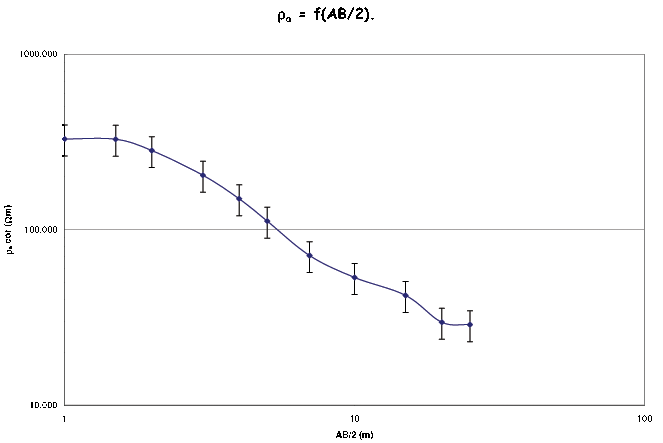
For the vertical prospection, the measure take place at the common point between vertical ligne in the middle of the electrode and the half-circle passing by electrodes A and B. The measure depth is AB/2.
We exploit data with a software. The software needs the number of layers. For each layer, the software needs thickness and resisitivity. A theorical graphe is drawn by the software. Then, we just have to compare the two graphes and adjust parameters in order to obtain an interpretation of the data.
There are also equipement with many electrodes, which can make vertical and horizontal measure in the same time. This kind of equipement gives data in sections.
<<< Graphe ρ=f(AB/2) obtain with vertical measure (logarithmic axis).
| Top of the page | Home |
Radar prospection allow to obtain an image of the soil in depth. A radar wave is send in the soil. It reflects itself on objects like pipes or geological layers, after it is picked up by an antenna. The movement of the radar's source and antenna allow us to obtain a picture of the soil.
| Top of the page | Home |
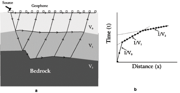
Sisimical prospection use the properties of sismic waves. Some sensors (geophones) are lined up with regular gap. At an extremity of the line, a source send waves. Sources can be a hammer blow, an explosion or vibrater truck. The source is changing with the lenght of the line and the depth we want to measure. Sismic waves are capted by geophones. The study of the first arrival time at each geophone give us some informations about the nature of the soil. Two kinds of measurements are possible: reflection and refraction. Refraction measurement is illustrated opposite. The source is fixed. In the graphe (b), black points symbolise the first arrival of waves at the geophone. The points are correlated theirself with lines. Each line is carateristic of a layer. The slope of the line is the inverse of the wave's propagation speed in the layer.
Illustration of sismic refraction. (a) Theorical section and ways of sismic waves from source to geophone. (b) This graphe represent the first arrival time as fonction of the source's distance. >>>
For the sismic reflection, the source is moving along the line near each geophone. The line wich is registered is the wave which travels perpendiculary to the geophone. The wave reflectes herself on the different geological layers (reflecters) and returns to the geophone. On the graphe (sismographe), reflecters appear like peaks. If we move source along the geophone's line, we obtain many sismographes where the reflecters appears. We place the whole sismographe one near other and we obtain a section of the soil.
| Top of the page | Home |

For the gravimetric prospection, we use Earth's gravity field properties in order to search density's anomaly. A gravimeter measures gravity g. Many corrections are necessarely before having interpretable data:
<<< gravimetric anomaly example. (a) Topography, (b) topographical anomaly, (c) Bouguer anomaly.
We present here measurement from a line accross an old castel and accross two moats (topographical depression).The Bouguer anomaly is positive between the two moats. There might be objects with higher density than around in depth. That's for example, castel's foundations.
| Top of the page | Home |

Magnetic prospection use the properties of the magnetic field and the magnetic gradient of the Earth. If an object with magnetic susceptibility buried, it will change the local magnetic field and it will create an anomaly. A magnetometer has two sensors one above the other, with a known gap. With one sensor we can have a measurement of the magnetic field. If we substract the measure of the higher sensor to the measure of the other sensor we obtain the magnetic gradient.
Like in gravimetry, we have to make correction in order to have interpretable data. Earth's magnetic field change in time. We must substract these variations. There are 2 solutions : first, we put a second magnetometer in a area far away which record the magnetic field continously, second, we take measure of Earth's magnetic field from a geomagnetic observatory.
In this example, an iron bar is buried in the center of the field. It causes a positive anomaly in South, and a negative anomaly in North. We can observe this anomaly in both map : anomaly and gradient.
Magnetic anomaly map (left) and magnetic gradient map (right). White points symbolyse mesure points.>>>
| Top of the page | Home |